Decomposition of KL_Pred
Published:
Notations
Let us consider a training dataset $\mathcal{D}$ consisting of $N$ i.i.d. samples,
\[\begin{equation*} \mathcal{D}= \{ (\boldsymbol{x}_i, y^*_i) \}_{i=1}^N \in (\mathcal{X} \times \mathcal{Y})^N \end{equation*}\]where $\mathcal{X}$ represents the input space and $\mathcal{Y}={1,\ldots,K}$ is a set of labels.
Samples drawn from $\mathcal{D}$ follow an unknown conditional probability distribution $p(\mathbf{y} \vert \mathbf{x})$ where $\mathbf{x}$ and $\mathbf{y}$ are random variables over input space and label space respectively.
Let $f^{\boldsymbol{\theta}}: \mathcal{X} \rightarrow \mathcal{X’}$ be a neural network (NN) parametrized by $\boldsymbol{\theta}$ where $\mathcal{X’} = \mathbb{R}^K$ is the logit space. We consider categorical probabilities over labels as random variable $\mathbf{z}$.
Following (Malinin & Gales, 2018), a NN explicitly parametrizes a distribution $p_{\theta}(\mathbf{z} \vert \mathbf{x})$ over categorical probabilities on a simplex. For its conjugate properties with categorical distributions, we chose to model $p_{\theta}(\mathbf{z} \vert \mathbf{x})$ as a Dirichlet distribution whose concentration parameters $\boldsymbol{\alpha}(\boldsymbol{x}, \boldsymbol{\theta}) = \exp (f^{\boldsymbol{\theta}}(\boldsymbol{x}))$ are given by the output of the NN: \begin{equation} p_{\theta}(\mathbf{z} \vert \mathbf{x} = \boldsymbol{x}) = \mathrm{Dir} \big ( \mathbf{z} \vert \boldsymbol{\alpha}(\boldsymbol{x}, \boldsymbol{\theta}) \big ) = \frac{\Gamma(\alpha_0 (\boldsymbol{x}, \boldsymbol{\theta}))}{\prod_c \Gamma(\alpha_c(\boldsymbol{x}, \boldsymbol{\theta}))} \prod_{c=1}^K z_j^{\alpha_c(\boldsymbol{x}, \boldsymbol{\theta}) - 1} \end{equation} where $\Gamma$ is the Gamma function, $\forall c \in \mathcal{Y}, \alpha_j > 0$ , $\alpha_0 = \sum_c \alpha_c$ and $\sum_c z_c$ = 1 such that $\mathbf{z}$ lives in the $(K-1)$-dimensional unit simplex $\triangle^{K-1}$.
$\textrm{KL}_{\textrm{Pred}}$ criterion
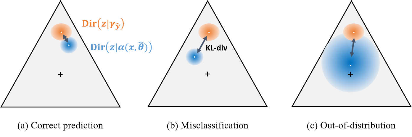
We propose an uncertainty criterion, denoted $\textrm{KL}_{\textrm{Pred}}$, which measures the KL-divergence between NN’s output and a sharp Dirichlet distribution with concentration parameters $\boldsymbol{\gamma}_{\hat{y}}$ focused on the predictive class $\hat{y}$:
\[\begin{equation} \textrm{KL}_{\textrm{Pred}}(\boldsymbol{x}) = \textrm{KL} \Big ( \textrm{Dir} \big (\mathbf{z} \vert \boldsymbol{\alpha}(\boldsymbol{x}, \boldsymbol{\hat{\theta}}) \big ) ~\vert \vert~ \textrm{Dir} \big ( \mathbf{z} \vert \boldsymbol{\gamma}^{\hat{y}} \big ) \Big ) \end{equation}\]To ensure an accurate estimation of concentration parameters $\boldsymbol{\gamma}^{\hat{y}}$, we compute the empirical exponential logits mean of the predicted class $\hat{y}$ on training set $\mathcal{D}$:
\[\begin{equation*} \boldsymbol{\gamma}^{\hat{y}} = \frac{1}{N^{\hat{y}}} \sum_{i: y_i=\hat{y}}^N \boldsymbol{\alpha}(\boldsymbol{x_i}, \boldsymbol{\hat{\theta}}), \quad \quad \textrm{with}~~ \boldsymbol{\alpha}(\boldsymbol{x_i}, \boldsymbol{\hat{\theta}}) = \exp (f^{\boldsymbol{\hat{\theta}}}(\boldsymbol{x}_i)) \end{equation*}\]where $N^{\hat{y}}$ is the number of training samples with label $\hat{y}$.

The lower $\textrm{KL}_{\textrm{Pred}}$ is, the more certain we are in the prediction. Previous figure illustrates the fact that correct predictions will have Dirichlet distributions similar to the computed mean distribution for the predicted class, and thus associated with a low uncertainty measure. Misclassified predictions are expected to present different concentration parameters than the average computed on training set resulting in a higher $\textrm{KL}_{\textrm{Pred}}$ measure. In comparison, differential entropy is not adequate when it comes to detect misclassifications (Malinin & Gales, 2018) as it corresponds to measuring the KL-divergence of the model’s output and the maximum-entropy distribution, which is the uniform distribution on a simplex.
Decomposition into aleatoric and epistemic uncertainty
We note that $\textrm{KL}_{\textrm{Pred}}$ corresponds to the definition of reverse KL-divergence loss (Malinin & Gales, 2019). It can be decomposed into the reverse cross-entropy and the negative differential entropy:
\[\begin{equation} \textrm{KL}_{\textrm{Pred}}(\boldsymbol{x}) = \underbrace{\mathbb{E}_{p \big ( \mathbf{z} \vert \boldsymbol{\alpha}(\boldsymbol{x}, \boldsymbol{\hat{\theta}}) \big )} \Big [- \log \textrm{Dir} \big ( \mathbf{z} \vert \boldsymbol{\gamma}_{\hat{y}} \big ) \Big ]}_\text{Reverse Cross-Entropy} - \underbrace{\mathcal{H} \Big [ \textrm{Dir} \big (\mathbf{z} \vert \boldsymbol{\alpha}) \big ) \Big ]}_\text{Differential Entropy} \end{equation}\](Note we ommit the dependence in $\boldsymbol{x}$ and $\boldsymbol{\hat{\theta}}$ in $\boldsymbol{\alpha}(\boldsymbol{x},\boldsymbol{\hat{\theta})}$ for clarity.)
First, the differential entropy can be written as the negative KL-divergence between NN’s output and the uniform Dirichlet distribution $\mathcal{U}(1)$:
\[\begin{equation} \mathcal{H} \Big [ \textrm{Dir} \big (\mathbf{z} \vert \boldsymbol{\alpha}) \big ) \Big ] = - \textrm{KL} \Big ( \textrm{Dir} \big (\mathbf{z} \vert \boldsymbol{\alpha}) \big ) ~\vert \vert~ \textrm{Dir} \big ( \mathbf{z} \vert \mathcal{U}(1) ) \Big ) \end{equation}\]As stated in (Malinin & Gales, 2019; Nandy et al., 2020), the differential entropy measures the epistemic uncertainty.
When considering the reverse cross-entropy (RCE) term:
\[\begin{align*} \textrm{RCE} &= \mathbb{E}_{p \big ( \mathbf{z} \vert \boldsymbol{\alpha} \big )} \Big [- \log \textrm{Dir} \big ( \mathbf{z} \vert \boldsymbol{\gamma}^{\hat{y}} \big ) \Big ] \\ &= - \log \Gamma(\boldsymbol{\gamma}^{\hat{y}}_0) + \sum_{c=1}^K \log \Gamma(\boldsymbol{\gamma}^{\hat{y}}_c) + \sum_{c=1}^K (\boldsymbol{\gamma}^{\hat{y}}_c - 1) \mathbb{E}_{p \big ( \mathbf{z} \vert \boldsymbol{\alpha} \big )} \big [\log(\boldsymbol{z}_c)] \\ &= \big ( \log \Gamma(K) - \log \Gamma(\boldsymbol{\gamma}^{\hat{y}}_0) + \sum_{c=1}^K \log \Gamma(\boldsymbol{\gamma}^{\hat{y}}_c) \big ) + \sum_{c=1}^K (\boldsymbol{\gamma}^{\hat{y}}_c - 1)(\psi(\boldsymbol{\alpha}_0) - \psi(\boldsymbol{\alpha}_c)) \end{align*}\]The first term depends only on the fixed target distribution $\boldsymbol{\gamma}^{\hat{y}}$ while the second term also consider logits values through $\boldsymbol{\alpha}$.
Case 1: $\textrm{KL}_{\textrm{Pred}}$
We compute only the empirical exponential logit mean of the predicted class $\hat{y}$:
\[\begin{equation*} \boldsymbol{\gamma}^{(1)} = [\boldsymbol{\gamma}_1^{(1)},...,\boldsymbol{\gamma}_K^{(1)}] \quad \quad \textrm{with}~~ \boldsymbol{\gamma}_c^{(1)}= \begin{cases} \frac{1}{N^{\hat{y}}} \sum_{i: y_i=\hat{y}}^N \boldsymbol{\alpha}_c, &\text{if}\ c=\hat{y} \\ 1, &\ \text{else.} \end{cases} \end{equation*}\]Hence, we can simplify RCE as:
\[\begin{equation} \textrm{RCE}^{(1)} = \log \Gamma(K) - \log \Gamma(\boldsymbol{\gamma}_{\hat{y}}^{(1)}+K-1) + \log \Gamma(\boldsymbol{\gamma}_{\hat{y}}^{(1)}) + (\boldsymbol{\gamma}_{\hat{y}}^{(1)} - 1)(\psi(\boldsymbol{\alpha}_0) - \psi(\boldsymbol{\alpha}_{\hat{y}})) \end{equation}\]We obtain the following figures for the decomposition and $\textrm{KL}_{\textrm{Pred}}$ criterion:

Case 2: $\textrm{KL}_{\textrm{PredFull}}$
We compute the full empirical vector as defined in the introductive part:
\[\begin{equation*} \boldsymbol{\gamma}^{(2)} = \frac{1}{N^{\hat{y}}} \sum_{i: y_i=\hat{y}}^N \boldsymbol{\alpha} \end{equation*}\](Note that $\boldsymbol{\gamma}_{\hat{y}}^{(2)} = \boldsymbol{\gamma}_{\hat{y}}^{(1)}$.)
In this case, there is no simplification as done previously. However, we can further decompose:
\[\begin{equation} \textrm{RCE}^{(2)} = \textrm{RCE}^{(1)} + \Big (- \log \Gamma \big ( \sum_{c \neq \hat{y}} (\boldsymbol{\gamma}_c^{(2)}-1 \big ) + \sum_{c \neq \hat{y}} \big ( \log \Gamma(\boldsymbol{\gamma}_c^{(2)}) + (\boldsymbol{\gamma}_c^{(2)} - 1)(\psi(\boldsymbol{\alpha}_0) - \psi(\boldsymbol{\alpha}_c) \big ) \Big ) \end{equation}\]
References
- A. Malinin, & M. Gales. (2018). Predictive Uncertainty Estimation via Prior Networks. In Advances in Neural Information Processing Systems.
- A. Malinin, & M. Gales. (2019). Reverse KL-Divergence Training of Prior Networks: Improved Uncertainty and Adversarial Robustness. In Advances in Neural Information Processing Systems.
- J. Nandy, W. Hsu, & M.-L. Lee. (2020). Towards Maximizing the Representation Gap between In-Domain and Out-of-Distribution Examples. In Advances in Neural Information Processing Systems.
