
A Survey on Dirichlet Neural Networks
Published:
In the past few years, a variety of Dirichlet-based methods for classification have emerged in the machine learning community. Before going into a detailed review of these approaches, we introduce the Dirichlet-multinomial model, a classic problem in machine learning which will help to better understand the intution behind the method.
Table of contents
- Preliminaries: the Dirichlet-multinomial Model
- Dirichlet Neural Networks, a Bayesian Approach
- Prior Networks
- Maximizing the Gap between In- and Out-distribution for Prior Networks
- Evidential Networks
- Generative Evidential Networks
- Variational Inference for Dirichlet Networks
- Posterior Networks, a Density-based Approach
- Summary and Discussion
Preliminaries: the Dirichlet-multinomial Model
Let us take the problem of infering the probability that a dice with $C$ sides comes up as face $c$.
This example is heavily inspired by Section 3.4 of (Murphy, 2013)’s book.
Suppose we observe $N$ dice rolls. As we always roll the same dice, our training dataset consists of \(\mathcal{D} = \{(x, y^{(i)})\}_{i=1}^N\) where \(y^{(i)} \in \{1,...,C\}\). If we assume data is i.i.d, the likelihood has the form:
\[\begin{equation} p(\mathcal{D} \vert \boldsymbol{\pi}) = \mathrm{Cat}(\mathcal{D} \vert \boldsymbol{\pi}) = \prod_{c=1}^C \pi_c^{N_c} \label{eq:likelihood_multinomial} \end{equation}\]where \(N_c = \sum_{i=1}^N \mathbb{I}(y^{(i)} = c)\) is the number of observations of class $c$ among the $N$ dice rolls (sufficient statistics).
For its conjugate properties with categorical distributions, we chose to model the prior as a Dirichlet distribution with concentration parameters $\boldsymbol{\beta}$:
\[\begin{equation} p(\boldsymbol{\pi}) = \mathrm{Dir} \big (\boldsymbol{\pi} ; \boldsymbol{\beta} \big ) = \frac{\Gamma(\beta_0)}{\prod_{c=1}^C \Gamma(\beta_c)} \prod_{c=1}^C \pi_c^{\beta_c- 1} \end{equation}\]Multiplying the likelihood by the prior, we find that the posterior is also a Dirichlet distribution:
\[\begin{align} p(\boldsymbol{\pi} \vert \mathcal{D}) &\propto p(\mathcal{D} \vert \boldsymbol{\pi}) p(\boldsymbol{\pi}) \\ &\propto \prod_{c=1}^C \pi_c^{N_c} \pi_c^{\beta_c - 1} \\ &= \mathrm{Dir} \big (\boldsymbol{\pi} \vert \beta_1 + N_1,..., \beta_C + N_C \big ) \end{align}\]Now, what we really care about is to compute the posterior predictive distribution for a single multinouilli trial:
\[\begin{align} P(y=c \vert \mathcal{D}) &= \int P(y=c \vert \boldsymbol{\pi}) p(\boldsymbol{\pi} \vert \mathcal{D}) d\boldsymbol{\pi} \\ &= \int \pi_c \cdot p(\boldsymbol{\pi} \vert \mathcal{D}) d\boldsymbol{\pi} \\ &= \mathbb{E}_{p(\boldsymbol{\pi} \vert \mathcal{D})} \big [\pi_c] = \frac{\beta_c + N_c}{\beta_0 + N} \end{align}\]We observe that the prior distribution acts as a Bayesian smoothing by adding pseudo-count $\boldsymbol{\beta}$ to the true count.
Consider $A,B$ two random variables with respective realisations $a,b$. In this blog post, we use the abusive notation \(\mathbb{E}_{p(a \vert b)} \big [ f(a) \big ] = \int f(a) p(A=a \vert B=b) da~\) instead of \(~\mathbb{E} \big [f(a) \vert B=b \big ]\) for conciseness.
Dirichlet Neural Networks, a Bayesian Approach
We extend the Bayesian treatment of a single categorical distribution to classification. In classification tasks, we predict the class label $y_i$ from a different categorical distribution for each input $\boldsymbol{x}_i$. Dataset consists of a collection of i.i.d training samples \(\mathcal{D} = \{(\boldsymbol{x}^{(i)}, y^{(i)})\}_{i=1}^N \in (\mathcal{X} \times \mathcal{Y})^N\) where $\mathcal{X}$ represents the input space and \(\mathcal{Y}=\{1,\ldots,C\}\) is a set of class labels. Samples drawn from $\mathcal{D}$ follow an unknown joint probability distribution $p(\boldsymbol{x}, y)$ where $\boldsymbol{x}$ and $y$ are random variables over input space and label space respectively.
Let us denote $\boldsymbol{\pi} =[\pi_1,…,\pi_C]$ the random variable over categorical probabilities. The likelihood given a sample $\boldsymbol{x}$ has the form:
\[\begin{equation} y \vert \boldsymbol{\pi}, \boldsymbol{x} \sim \mathrm{Cat}(y \vert \boldsymbol{\pi}, \boldsymbol{x}) = \prod_{c=1}^C \pi_c^{\tilde{N}_c(\boldsymbol{x})} \end{equation}\]The difference with Eq.(\ref{eq:likelihood_multinomial}) is that \(\tilde{N}_c(\boldsymbol{x})\) now represents a label frequency count at point \(\boldsymbol{x}\).
Most of the time, the estimator \(\tilde{N}_c(\boldsymbol{x})\) uses single or very few samples since most of the inputs are unique or very rare in the training set.
Obviously, for an unknown test sample \(\boldsymbol{x}^*\), we don’t have access to its label frequency count when infering. Consequently, we are not able to estimate the posterior predictive distribution:
\[\begin{align} P(y =c \vert \boldsymbol{x^*}, \mathcal{D}) &= \int P(y=c \vert \boldsymbol{\pi}, \boldsymbol{x^*}) p(\boldsymbol{\pi} \vert \boldsymbol{x}^*, \mathcal{D}) d\boldsymbol{\pi} \\ &= \mathbb{E}_{p(\boldsymbol{\pi} \vert \boldsymbol{x}^*, \mathcal{D})} \big [ \pi_c \big ] \end{align}\]Approaches like ensembles (Lakshminarayanan et al., 2017) and dropout (Gal & Ghahramani, 2016) model implicity the posterior distribution over categorical probabilities by marginalizing over the network parameters $\boldsymbol{\theta}$ and estimate the predictive distribution thanks to Monte-Carlo Sampling:
\[\begin{equation*} P(y=c \vert \boldsymbol{x}^*, \mathcal{D}) = \int P(y=c \vert \boldsymbol{x}^*, \boldsymbol{\theta}) p(\boldsymbol{\theta} \vert \mathcal{D}) d\boldsymbol{\theta} \approx \frac{1}{S} \sum_{s=1}^S P(y=c \vert \boldsymbol{x}^*, \boldsymbol{\theta}_s) \end{equation*}\]With Dirichlet models, we now explicitly parametrizes the distribution over the predictive categorical $p(\boldsymbol{\pi} \vert \boldsymbol{x}^*, \mathcal{D})$ with a Dirichlet distribution. This effectively emulate an ensemble without sampling approximation, thanks a closed-form solution which also requires one forward pass only.
In particular, Dirichlet modelisation enables to distinctly account for the aleatoric uncertainty and the epistemic uncertainty of a prediction. The aleatoric uncertainty is irreducible from the data due to class overlap or noise, e.g. a fair coin has 50/50 chance for head. The epistemic uncertainty is due to the lack of knowledge about unseen data, e.g. an image of an unknown object or an outlier in the data.
Epistemic uncertainty relates to the spread of the categorical distribution \(p(\boldsymbol{\pi} \vert \boldsymbol{x}^*, \mathcal{D})\) on the simplex, which corresponds to \(\alpha_0 = \sum_{c=1}^C \alpha_c\) for a Dirichlet distribution. Aleatoric uncertainty is linked to the position of the mean on the simplex. Equipped with this configuration, we would like Dirichlet network to yield the desired behaviors shown in the figure below:
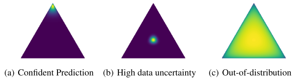
When the model is confident in its prediction, it should yield a sharp distribution centered on one of the corners of the simplex (Fig a.). For an input in a region with high degrees of noise or class overlap (aleatoric uncertainty), it should yield a sharp distribution focused on the center of the simplex, which corresponds to being confident in predicting a flat categorical distribution over class labels (Fig b.). Finally, for out-of-distribution inputs, the Dirichlet network should yield a flat distribution over the simplex, indicating large epistemic uncertainty (Fig c.).
Now the remaining questions are:
- How to induce such desired behavior when training Dirichlet networks?
- What measure should we use for each type of uncertainty?
In the recent literature, (Malinin & Gales, 2018) and (Sensoy et al., 2018) simultaneously proposed to learn a Dirichlet neural network to better represent uncertainty in classification. Following papers (Malinin & Gales, 2019; Chen et al., 2019; Sensoy et al., 2020; Joo et al., 2020; Nandy et al., 2020; Charpentier et al., 2020) build on this framework by improving learning. In the rest of this post, we will review these approaches and their benefits.
Prior Networks
(Malinin & Gales, 2018) propose to model the concentration parameters $\boldsymbol{\alpha}$ of the distribution over probabilities $p(\boldsymbol{\pi} \vert \boldsymbol{x}^*; \boldsymbol{\boldsymbol{\hat{\theta}}}) = \mathrm{Dir} \big (\boldsymbol{\pi} \vert \boldsymbol{\alpha} \big )$ where the concentration parameters $\boldsymbol{\alpha}$ are computed by the output of a neural network $f$.
By marginalizing network parameters $\boldsymbol{\theta}$, the distribution over probabilities writes as follow:
\[\begin{equation*} p(\boldsymbol{\pi} \vert \boldsymbol{x^*}, \mathcal{D}) = \int p(\boldsymbol{\pi} \vert \boldsymbol{x^*}, \boldsymbol{\theta}) p(\boldsymbol{\theta} \vert \mathcal{D}) d\boldsymbol{\theta} \end{equation*}\]For simplicity, authors assume a Dirac-delta approximation of the parameters
\[\begin{equation*} p(\boldsymbol{\theta} \vert \mathcal{D}) = \delta(\boldsymbol{\theta} - \boldsymbol{\hat{\theta}}) \Rightarrow p(\boldsymbol{\pi} \vert \boldsymbol{x^*}, \mathcal{D}) \approx p(\boldsymbol{\pi} \vert \boldsymbol{x^*}; \boldsymbol{\hat{\theta}}) \end{equation*}\]The posterior over class labels will be given by the mean of the Dirichlet:
\[\begin{equation} P(y=c \vert \boldsymbol{x}^*, \mathcal{D}) = \int P(y=c \vert \boldsymbol{\pi}, \boldsymbol{x^*}) p(\boldsymbol{\pi} \vert \boldsymbol{x^*}; \boldsymbol{\hat{\theta}}) = \frac{\alpha_c}{\alpha_0} \end{equation}\]If an exponential output function is used, i.e $\alpha_c = e^{f_c(\boldsymbol{x^*}, \boldsymbol{\hat{\theta}})}$, then the expected posterior probability of a label $c$ is given by the output of the softmax:
\[\begin{equation} P(y=c \vert \boldsymbol{x^*}, \mathcal{D}) = \frac{e^{f_c(\boldsymbol{x^*}, \boldsymbol{\hat{\theta}})}}{\sum_{k=1}^C e^{f_k(\boldsymbol{x^*}; \boldsymbol{\hat{\theta}})}} \end{equation}\]The representation is similar to standard neural networks for classification with the difference that the output now describes the concentration parameters of a Dirichlet distribution over a simplex.
Learning
Merely training with a cross-entropy loss only affects the value of the concentration parameters $\alpha_y$ associated to the true class. It does not enable to control the spread parameter $\alpha_0$ of the Dirichlet distribution over categorical probabilities.
For clarity, we introduce the existence of out-of-domain training data \(\mathcal{D}_{\textrm{out}}\) and now denotes the training dataset by \(\mathcal{D}_{\textrm{in}}\). Associated random variable specifying whether a sample belong to in-distribution or out-distribution takes values in \(\{i,o\}\).
To enforce the desired behavior for out-of-distribution (OOD) samples, (Malinin & Gales, 2019) propose a reverse KL-divergence-based contrastive loss between in-distribution and out-distribution samples. It consists of minimizing the reverse KL divergence between the neural network’s output and a sharp Dirichlet distribution focused on the appropriate class for in-distribution data, and between the output and a flat Dirichlet distribution for out-of-distribution data:
\[\begin{align} \mathcal{L}_{\textrm{RKL-PN}}(\boldsymbol{\theta}) &= \mathbb{E}_{p(\boldsymbol{x})} \Big [ \textrm{KL} \big ( \textrm{Dir} ( \boldsymbol{\pi} \vert \boldsymbol{x}, \boldsymbol{\theta} ) ~\vert \vert~ \textrm{Dir} ( \boldsymbol{\pi} \vert \bar{\boldsymbol{\beta}}) \big ) \Big ] \\ &=\mathbb{E}_{p(\boldsymbol{x})} \Big [\sum_{c=1}^C P(y=c \vert \boldsymbol{x}) \cdot \textrm{KL} \big ( \textrm{Dir} ( \boldsymbol{\pi} \vert \boldsymbol{x}, \boldsymbol{\theta} ) ~\vert \vert~ \textrm{Dir} ( \boldsymbol{\pi} \vert \boldsymbol{\beta}^{(c)}) \big ) \Big ] \\ &=\mathbb{E}_{p(\boldsymbol{x} \vert i)} \Big [\sum_{c=1}^C P(y=c \vert \boldsymbol{x}) \cdot \textrm{KL} \big ( \textrm{Dir} ( \boldsymbol{\pi} \vert \boldsymbol{x}, \boldsymbol{\theta} ) ~\vert \vert~ \textrm{Dir} ( \boldsymbol{\pi} \vert \boldsymbol{\beta}^{(c)}_{\textrm{in}}) \big ) \Big ] P(i) \\ &~~~~~~+ \mathbb{E}_{p(\boldsymbol{x} \vert o)} \Big [\sum_{c=1}^C P(y=c \vert \boldsymbol{x}) \cdot \textrm{KL} \big ( \textrm{Dir} ( \boldsymbol{\pi} \vert \boldsymbol{x}, \boldsymbol{\theta} ) ~\vert \vert~ \textrm{Dir} ( \boldsymbol{\pi} \vert \boldsymbol{\beta}^{(c)}_{\textrm{out}}) \big ) \Big ] P(o) \nonumber \end{align}\]where \(\bar{\boldsymbol{\beta}} = \sum_{c=1}^C P(y=c \vert \boldsymbol{x}) \cdot \boldsymbol{\beta}^{(c)}\) is an arithmetic mixture of the target concentration parameters for each class.
We approximate with the empirical distributions \(\hat{p}(X \vert i)\) on \(\mathcal{D}_{\textrm{in}}\) and \(\hat{p}(X \vert o)\) on \(\mathcal{D}_{\textrm{out}}\), which boils down to minimize the following loss:
\[\begin{align} \hat{\mathcal{L}}_{\textrm{RKL-PN}}(\boldsymbol{\theta}, \mathcal{D}_{\textrm{in}}, \mathcal{D}_{\textrm{out}})= \sum_{i=1}^{N_i} &~\textrm{KL} \Big ( \textrm{Dir} \big ( \boldsymbol{\pi} \vert \boldsymbol{x}^{(i)}, \boldsymbol{\theta} \big ) ~\vert \vert~ \textrm{Dir} \big ( \boldsymbol{\pi} \vert \boldsymbol{\beta}_{\textrm{in}}^{(i)} \big ) \Big ) \\ &+ \gamma \sum_{j=1}^{N_o} \mathrm{KL} \Big ( \textrm{Dir} \big ( \boldsymbol{\pi} \vert \boldsymbol{x}^{(j)}, \boldsymbol{\theta} \big ) ~\vert \vert~ \textrm{Dir} \big ( \boldsymbol{\pi} \vert \boldsymbol{\beta}_{\textrm{out}}^{(j)} \big ) \Big ) \nonumber \end{align}\]where in-domain target concentrations parameters are \(\boldsymbol{\beta}_{\textrm{in}}^{(i)}\) are such that \(\forall c\neq y^{(i)}, \boldsymbol{\beta}^{(i)}_{c, in}=1\) and \(\boldsymbol{\beta}^{(i)}_{y, in} = 1 + B\), with $B$ a hyperparameter. A flat uniform Dirichlet is chosen for out-domain target distribution : \(\forall c, \boldsymbol{\beta}_{c,\textrm{out}}^{(j)}=1\). Hyperparameter $\gamma = \hat{P}(o) / \hat{P}(i)$ helps to balance the out-of-distribution loss weight in training.
Authors chose $B=100$ to aim for in-domain distributions with high target concentration parameters.
Measuring uncertainty
(Malinin & Gales, 2018) consider measures from the expected predictive categorical distribution \(p(y \vert \boldsymbol{x^*}, \mathcal{D})\) as a mesure of total uncertainty. This includes the Maximum Class Probability (MCP) and the predictive entropy \(\mathcal{H} \big [y \vert \boldsymbol{x^*}, \mathcal{D}]\).
Based on (Depeweg et al., 2018), they decompose the predictive entropy into two terms :
\[\begin{equation} \underbrace{\mathcal{H} \Big [ \mathbb{E}_{p(\boldsymbol{\pi} \vert \boldsymbol{x^*}; \hat{\boldsymbol{\theta}})} \big [ p(y \vert \boldsymbol{\pi}) \big] \Big ]}_{\text{Total Uncertainty}} = \underbrace{\mathbb{E}_{p(\boldsymbol{\pi} \vert \boldsymbol{x^*}; \hat{\boldsymbol{\theta}})} \Big [ \mathcal{H} \big [ p(y \vert \boldsymbol{\pi}) \big] \Big]}_{\text{Expected Aleatoric Uncertainty}} + \underbrace{\mathcal{MI} \Big [y, \boldsymbol{\pi} \vert \boldsymbol{x^*}; \hat{\boldsymbol{\theta}} \Big ]}_{\text{Epistemic Uncertainty}} \end{equation}\]- \(\mathcal{MI} \Big [y, \boldsymbol{\pi} \vert \boldsymbol{x^*}; \hat{\boldsymbol{\theta}} \Big ]\) is the mutual information between class label and categorical probabilities from the posterior. It corresponds to a measure of the spread of the posterior distribution \(p(\boldsymbol{\pi} \vert \boldsymbol{x^*}; \hat{\boldsymbol{\theta}})\)
- \(\mathbb{E}_{p(\boldsymbol{\pi} \vert \boldsymbol{x^*}; \hat{\boldsymbol{\theta}})} \Big [ \mathcal{H} \big [ p(y \vert \boldsymbol{\pi}) \big] \Big]\) is the expected entropy of the categorical distribution.
When dealing with ensemble methods, the expected entropy of the categorical distribution is computed with the Monte Carlo estimates. With Dirichlet networks, there is a closed-form.
In their experiments, they use the mutual information \(\mathcal{MI}\) to detect out-of-distribution samples and MCP for misclassification detection.
Maximizing the Gap between In- and Out-distribution for Prior Networks
(Nandy et al., 2020) motivate their work by showing that using the reverse KL-divergence tends to produce flatter Dirichlet distributions for in-domain misclassified examples. As a consequence, this effect may harden the goal of making in-domain and out-domain samples distinguishable.
To demonstrate this behavior, they decompose the KL-divergence into the reverse cross-entropy and the differential entropy:
\[\begin{align} \mathcal{L}_{\textrm{RKL-PN}}(\boldsymbol{\theta}) &= \mathbb{E}_{p(\boldsymbol{x})} \Big [ \textrm{KL} \big ( \textrm{Dir} ( \boldsymbol{\pi} \vert \boldsymbol{x}, \boldsymbol{\theta} ) ~\vert \vert~ \textrm{Dir} ( \boldsymbol{\pi} \vert \boldsymbol{\bar{\beta}}) \big ) \Big ] \\ &= \mathbb{E}_{p(\boldsymbol{x})} \Big [ \underbrace{\mathbb{E}_{p( \boldsymbol{\pi} \vert \boldsymbol{x}, \boldsymbol{\theta})} \big [- \log \textrm{Dir} \big ( \boldsymbol{\pi} \vert \boldsymbol{\bar{\beta}}) \big ]}_\text{Reverse Cross-Entropy} - \underbrace{\mathcal{H} \big [ \textrm{Dir} \big (\boldsymbol{\pi} \vert \boldsymbol{x}, \boldsymbol{\theta}) \big ] \Big ]}_\text{Differential Entropy} \label{eq:reverse-kl} \end{align}\]Minimizing the differential entropy always leads to produce a flatter distribution. Hence, \(\mathcal{L}_{\textrm{RKL-PN}}\) relies only on the reverse cross-entropy to produce sharper distributions. This latter term can be derived as:
\[\begin{align} \mathbb{E}_{p( \boldsymbol{\pi} \vert \boldsymbol{x}, \boldsymbol{\theta})} \big [- \log \textrm{Dir} \big ( \boldsymbol{\pi} \vert \bar{\boldsymbol{\beta}}) \big ] &= \sum_{c=1}^C P(y=c \vert \boldsymbol{x}) (1 + B - 1)(\psi(\alpha_0) - \psi(\alpha_c)) \\ &= B\cdot \psi(\alpha_0) - \sum_{c=1}^C B \cdot P(y=c \vert \boldsymbol{x})\psi(\alpha_c) \label{eq:rce} \end{align}\]We can see in Eq.(\ref{eq:rce}) that the reverse cross-entropy term maximizes $\psi(\alpha_c)$ for each class $c$ with the factor $B \cdot P(y=c \vert \boldsymbol{x})$, while minimizing $\psi(\alpha_c)$ with the factor $B$. Imagine a sample with high aleatoric uncertainty, the reverse cross-entropy will leads to smaller concentration parameters $\boldsymbol{\alpha}$ than a confident sample.
The proposed solution is to force OOD samples to have even more lower concentration parameters, ideally \(\boldsymbol{\alpha}_{\textrm{out}} \rightarrow 0\).
Learning
Looking at the reverse cross-entropy term in Eq.(\ref{eq:rce}), a first solution could be to modify the target \(\beta_{\text{out}}\) within the reverse KL-divergence. Currently, \(\beta_{\text{out}}=1\) for OOD samples. Setting \(\beta_{\text{out}}>1\) would minimize $\alpha_0$ but also maximises individual concentration parameters $\alpha_c$. Conversely, $\beta_{\text{out}} \in [0,1[$ maximises $\alpha_0$ while minimizing $\alpha_c$’s. Eithier choice of $\beta_{\text{out}}$ may lead to uncontrolled values.
Instead, (Nandy et al., 2020) propose a new loss for Dirichlet Networks based on the usual cross-entropy loss and a explicit regularization on the concentration parameters:
\[\begin{align} \mathcal{L}_{\textrm{Max-PN}}(\boldsymbol{\theta}) = &\mathbb{E}_{p(\boldsymbol{x}, y \vert i)} \Big [ - \log p(y \vert \boldsymbol{x}, \boldsymbol{\theta}) - \frac{\lambda_{\textrm{i}}}{C} \sum_{c=1}^C \sigma(\alpha_c) \Big ] \\ &+ \gamma \cdot \mathbb{E}_{p(\boldsymbol{x},y \vert o)} \Big [ - \frac{1}{C} \sum_{c=1}^C \log P(y=c \vert \boldsymbol{x}, \boldsymbol{\theta}) - \frac{\lambda_{\textrm{o}}}{C} \sum_{c=1}^C \sigma(\alpha_c) \Big ] \nonumber \end{align}\]where \(\sigma\) the sigmoid function, \(\lambda_{\textrm{i}}\) and \(\lambda_{\textrm{o}}\) hyperparameters to control the precision of respective output distributions and \(\gamma = p(o)/p(i)\) balancing loss values between in- and out-domain distribution. Note that the term \(- \frac{1}{C} \sum_{c=1}^C \log P(y=c \vert \boldsymbol{x}, \boldsymbol{\theta})\) corresponds to minimise the cross-entropy with an uniform distribution.
To enforce negative values for OOD concentration parameters, authors chose \(\lambda_{\textrm{o}} = 1/C - 1/2 <0\). It leads the probability densities to be moved across the edges of the simplex to produce extremely sharp multi-modal distributions. They set \(\lambda_{\textrm{i}} = 1/2\) for in-domain examples.
Note that chosing \(\lambda_{\textrm{i}} = \lambda_{\textrm{o}} = 0\) leads to the same loss proposed in a non-Bayesian outlier exposure framework proposed by (Hendrycks et al., 2019)
Measuring uncertainty
As they explicitely regularize the logits, (Nandy et al., 2020) use \(\alpha_0 = \sum_c \alpha_c\) the sum of the concentration parameters of posterior distribution. In parallel, they also mention the differential entropy \(\mathcal{H} \big [ p( \boldsymbol{\pi} \vert \boldsymbol{x}, \hat{\boldsymbol{\theta}}) \big ]\), which is the entropy of the posterior distribution over probabilities :
\[\begin{equation} \mathcal{H} \big [ p( \boldsymbol{\pi} \vert \boldsymbol{x}, \hat{\boldsymbol{\theta}}) \big ] = \int p( \boldsymbol{\pi} \vert \boldsymbol{x}, \hat{\boldsymbol{\theta}}) \log p( \boldsymbol{\pi} \vert \boldsymbol{x}, \hat{\boldsymbol{\theta}}) d\boldsymbol{\pi} \end{equation}\]In particular, the differential entropy is equivalent to measuring the KL-divergence between the posterior distribution and a Dirichlet uniform \(\mathrm{Dir}(\boldsymbol{\pi} \vert \mathbf{u})\) where \(\forall c, u_c = 1\).
They measure OOD detection with mutual information or $\alpha_0$ and misclassification detection with MCP.
Evidential Networks
For now on, we will assume there is no OOD data available in training for the rest of the approaches presented below.
In a concurrent work to (Malinin & Gales, 2018), (Sensoy et al., 2018) also develop a Dirichlet-based model for neural network based on subjective logic (Josang, 2016) framework. Subjective logic formalizes the Dempster-Shafer theory’s notion of belief assignements over a frame of discernement as a Dirichlet distribution.
The Dempster-Shafer theory of evidence (Dempster, 2008) is a generalization of the Bayesian theory to subjective probabilities. It assigns belief masses to subsets of a frame of discernment, which denotes the set of exclusive possible states, e.g. possible class labels for a sample.
In practice, it boils down to account for an overall uncertainty mass of $u$ added to belief classes \(b_c\):
\[\begin{equation} u + \sum_{c=1}^C b_c = 1 \end{equation}\]where $u \geq 0$ and \(\forall c \in \mathcal{y}, b_c \geq 0\). A belief mass \(b_c\) for a singleton $c$ is computed using the evidence for the singleton. Let \(e_c \geq 0\) be the evidence derived for the $c^{th}$ singleton, then the belief \(b_c\) and the uncertainty $u$ are computed as:
\[\begin{equation} b_c = \frac{e_c}{S} \quad \textrm{and} \quad u = \frac{C}{S} \end{equation}\]where \(S = \sum_{c=1}^C (e_c +1)\). Note that the uncertainty is inversely proportional to the total evidence.
The link to Dirichlet distribution is as follow. Concentration parameters of distribution \(p(\boldsymbol{\pi} \vert \boldsymbol{x}, \boldsymbol{\theta})\) corresponds to evidences \(\alpha_c = e_c + 1\). Then, we obtain that \(S = \alpha_0\), which represents the spread of the distribution.
(Sensoy et al., 2018) propose to model the concentration parameters by a neural network output, hence:
\[\begin{equation} \boldsymbol{\alpha} = \textrm{ReLU} \big ( f(\boldsymbol{x}, \boldsymbol{\theta}) \big ) + 1 \end{equation}\]In contrast to previous work, they differs in the modelisation by replacing the softmax layer with an ReLU activation layer to ensure non-negative outputs.
Learning
Authors propose to train their Evidential Neural Network by minimizing the Bayes risk of the MSE loss with respect to the ‘class predictor’:
\[\begin{align} \mathcal{L}_{\textrm{ENN}}(\boldsymbol{\theta}) = \mathbb{E}_{p(\boldsymbol{x}, y)} \Big [\int \vert \vert \boldsymbol{y} - \boldsymbol{\pi} \vert \vert^2 \cdot p(\boldsymbol{\pi} \vert \boldsymbol{x}, \boldsymbol{\theta}) d\boldsymbol{\pi} + \lambda_t \cdot \textrm{KL} \big ( \textrm{Dir} ( \boldsymbol{\pi} \vert \tilde{\boldsymbol{\alpha}} ) ~\vert \vert~ \textrm{Dir} (\boldsymbol{\pi} \vert \mathbf{u}) \big ) \Big ] \end{align}\]Added to the Bayes risk, they also incorporate a KL-divergence regularization term which penalize ‘unknown’ predictive distributions. $\boldsymbol{y}$ denotes the one-hot representation of $y$, \(\textrm{Dir} (\boldsymbol{\pi} \vert \mathbf{u})\) is the Dirichlet uniform distribution and \(\tilde{\boldsymbol{\alpha}} = \boldsymbol{y} + (1- \boldsymbol{y}) \odot \boldsymbol{\alpha}\) is the Dirichlet parameters after removal of the non-misleading evidence from predicted parameters $\boldsymbol{\alpha}$. In the paper, \(\lambda_t = \min (1, t/10) \in [0, 1]\) is an annealing coefficient, with $t$ is the index of the current training epoch.
In particular, they also provide some interesting theoretical properties the Bayes risk minimization with MSE loss thanks to the variance identity:
\[\begin{align} \int \vert \vert \boldsymbol{y} - \boldsymbol{\pi} \vert \vert^2 \cdot p(\boldsymbol{\pi} \vert \boldsymbol{x}, \boldsymbol{\theta}) d\boldsymbol{\pi} &= \mathbb{E}_{p( \boldsymbol{\pi} \vert \boldsymbol{x}, \boldsymbol{\theta})} \Big [(\boldsymbol{y} - \boldsymbol{\pi})^2 \Big ] \\ &= \mathbb{E}_{p( \boldsymbol{\pi} \vert \boldsymbol{x}, \boldsymbol{\theta})} \Big [\boldsymbol{y} - \boldsymbol{\pi} \Big ]^2 + \textrm{Var} \Big [ \boldsymbol{y} - \boldsymbol{\pi} \Big ] \\ &= \sum_{c=1}^C (y_c - \alpha_c / \alpha_0)^2 + \frac{\alpha_c(\alpha_0 - \alpha_c)}{\alpha_0^2(\alpha_c + 1)} \end{align}\]The derivation decompose the loss into the first and second moments, which highlight it aims to achieve the joint goals of minimizing the prediction error and the variance of the Dirichlet distribution output by the neural network.
Measuring uncertainty
Without further reflection, (Sensoy et al., 2018) use predictive entropy \(\mathcal{H} \big [y \vert \boldsymbol{x^*}; \boldsymbol{\theta}]\) as uncertainty measure to be consistent with other approaches used in literature. Experiments include OOD detection and adversarial robustness.
Generative Evidential Networks
While, Evidential networks enable to account aleatoric and epistemic uncertainty separately, they fail to induce to desired behavior for out-of-distribution samples. There is no constraint on the out-distribution domain and models could still be able to derive large amount of evidence and become overconfident in their predictions for OOD samples.
To alleviate this issue, (Sensoy et al., 2020) extend their previous work and propose to synthetise out-of-distribution samples close to training samples thank to a generative model. Then, they learn a classifier using both types of samples and based on implicit density modeling to account for out-of-distribution samples during training.
Implicit density modeling
A convenient way to describe density of samples from a class $c$ is to describe it relative to the density of some other reference data. By using the same reference data for all classes in the training set, one desire to get comparable quantities for their density estimations. We reformulate the ratio between densities \(p(\boldsymbol{x} \vert y=c)\) and \(p(\boldsymbol{x} \vert o)\) as:
\[\begin{equation} \frac{p(\boldsymbol{x} \vert y=c)}{p(\boldsymbol{x} \vert o)} = \frac{P(y=c \vert \boldsymbol{x})}{p(o \vert \boldsymbol{x})} \frac{P(o)}{P(y=c)} \label{eq:density-ratio} \end{equation}\]where \(\frac{p(o)}{P(y=c)}\) can be approximated with the empirical count of samples of class $c$ and the empirical count of out-of-distribution training samples.
As shown in Eq.(\ref{eq:density-ratio}), one can approximate the log density ratio \(\log \frac{p(\boldsymbol{x} \vert y=c)}{p(\boldsymbol{x} \vert o)}\) as the logit output of a binary classifier (Lakshminarayanan & Mohamed, 2017), which is trained to discriminate between the samples from $P(y=c)$ and $P(o)$. Hence, along with the Dirichlet framework, each output \(f_c(\boldsymbol{x}, \boldsymbol{\theta})\) of a neural network classifier now also aims to approximate the log density ratio.
Concentration parameters are defined as \(\boldsymbol{\alpha} = e^{f(\boldsymbol{x}, \boldsymbol{\theta})} + 1\). If a sample $\boldsymbol{x}$ tends to be from out domain, then the density ratio should be close to zero, meaning almost zero evidence generated by the network for that sample.
Learning
Authors use the Bernoulli loss to train their network with a regularization term for misclassified samples:
\[\begin{align} \mathcal{L}_{\textrm{GEN}}(\boldsymbol{\theta}) = - \sum_{c=1}^C \Big (\mathbb{E}_{p(\boldsymbol{x} \vert c, i)} \big [&\log \sigma ( f_c(\boldsymbol{x}, \boldsymbol{\theta})) \big ] + \mathbb{E}_{p(\boldsymbol{x} \vert o)} \big [\log \big ( 1 - \sigma ( f_c(\boldsymbol{x}, \boldsymbol{\theta})) \big ) \big ] \Big ) \\ &+ \lambda \cdot \mathbb{E}_{p(\boldsymbol{x},y \vert i)} \Big [ \textrm{KL} \big ( \textrm{Dir} (\boldsymbol{\pi}_{-y} \vert \boldsymbol{\alpha}_{-y} )~\vert \vert~ \textrm{Dir} (\boldsymbol{\pi}_{-y} \vert \mathbf{u}) \big ) \Big ] \nonumber \end{align}\]where $\sigma$ is the sigmoid function, \(\boldsymbol{\pi}_{-y}\) and \(\boldsymbol{\alpha}_{-y}\) refers to the vector of probabilities \(\pi_c\) and the vector of concentration parameters \(\alpha_c\) such that \(c \neq y\). The regularization term aims to push concentration parameters of all classes $c \neq y$ to be close to uniform by minimizing a KL-divergence with the Dirichlet uniform distribution $\mathbf{u}$.
Finally, $\lambda$ is an sample-level hyperparameter controlling the weight of the regularization term. Authors defines $\lambda = 1 - \alpha_y / \alpha_0$, which is the expected probability of misclassification. Hence, when used as a weight of the KL-divergence term, it enables a learned loss attenuation: as the aleatoric uncertainty decreases, the weight of the regularization term decrease as well.
Note that this contrastive training is inspired from noise-constrative estimation (Gutmann & Hyvärinen, 2012) with the difference here that noisy data are generalized to out-of-distribution samples.
Generating out-of-distribution samples
To synthesize out-of-distribution samples, (Sensoy et al., 2020) relies on the latent space of a variational autoencoder (VAE) where they perturb in-domain sample representation with a multivariate Gaussian distribution. More precisely, for each $\boldsymbol{x}$ in training dataset, they sample a latent point $\boldsymbol{z}$ from the latent space distribution learned by a VAE and perturb it by \(\boldsymbol{\epsilon} \sim \mathcal{N}(\boldsymbol{0}, G(\boldsymbol{z}))\) where $G(\cdot)$ is a generative adversarial network (GAN) with non-negative output and adversarially trained against two discriminators (one that acts in the latent space, the other one in the input space). The VAE, generator and discriminators are iteratively trained until convergence.
Measuring uncertainty
As with Evidential Networks, (Sensoy et al., 2020) use predictive entropy \(\mathcal{H} \big [y \vert \boldsymbol{x^*}, \boldsymbol{\theta})]\) as uncertainty measure. Experiments include misclassification detection, OOD detection and adversarial robustness.
Variational inference for Dirichlet Networks
Using the Bayesian principle, the true posterior distribution over categorical distribution for a sample $(\boldsymbol{x}, y)$ can be obtained by:
\[\begin{equation} p(\boldsymbol{\pi} \vert \boldsymbol{x}, y) \propto p(y \vert \boldsymbol{\pi}, \boldsymbol{x}) p(\boldsymbol{\pi} \vert \boldsymbol{x}) \end{equation}\]Just as in the preliminaries for a Dirichlet-multinomial model, we define the prior \(p(\boldsymbol{\pi} \vert \boldsymbol{x})\) as a Dirichlet distribution with concentration parameters $\boldsymbol{\beta}$, which is conjugate to the categorical likelihood. Hence, we have the following posterior given dataset $\mathcal{D}$:
\[\begin{equation} p(\boldsymbol{\pi} \vert \boldsymbol{x},y) = \mathrm{Dir} \Big (\boldsymbol{\pi} \vert \beta_1 + \tilde{N}_1(\boldsymbol{x}),..., \beta_K + \tilde{N}_K(\boldsymbol{x}) \Big ) \label{eq:posterior_distribution} \end{equation}\]where \(\tilde{N}_c(\boldsymbol{x})\) now represents the empirical label frequency count at point \(\boldsymbol{x}\). Again, we see that the target posterior mean is explicitly smoothed by the prior belief. However, when predicting for a new sample $\boldsymbol{x}^*$, we obviously don’t know its label frequency.
(Joo et al., 2020) propose to approximate the posterior distribution with a variational distribution $q_{\boldsymbol{\theta}}(\boldsymbol{\pi} \vert \boldsymbol{x})$ modeled by the neural network’s output. They chose \(q_{\boldsymbol{\theta}}(\boldsymbol{\pi} \vert \boldsymbol{x})\) to be a Dirichlet distribution whose concentration parameters are \(\boldsymbol{\alpha} = e^{f(\boldsymbol{x}, \boldsymbol{\theta})}\).
Learning
In variational inference, the goal is to bring the variational distribution \(q_{\boldsymbol{\theta}}(\boldsymbol{\pi} \vert \boldsymbol{x})\) closer to the true posterior distribution \(p(\boldsymbol{\pi} \vert \boldsymbol{x}, y)\). In a standard way, (Joo et al., 2020), as well as (Chen et al., 2019), minimize the KL-divergence between the two distributions:
\[\begin{align} \mathrm{KL} \Big ( q_{\boldsymbol{\theta}}(\boldsymbol{\pi} \vert \boldsymbol{x})~\vert \vert~p(\boldsymbol{\pi} \vert \boldsymbol{x}, y) \Big ) &= \int q_{\boldsymbol{\theta}}(\boldsymbol{\pi} \vert \boldsymbol{x}) \log \frac{q_{\boldsymbol{\theta}}(\boldsymbol{\pi} \vert \boldsymbol{x})}{p(\boldsymbol{\pi} \vert \boldsymbol{x}, y)} \nonumber \\ &= \int q_{\boldsymbol{\theta}}(\boldsymbol{\pi} \vert \boldsymbol{x}) \log \frac{q_{\boldsymbol{\theta}}(\boldsymbol{\pi} \vert \boldsymbol{x}) p(y \vert \boldsymbol{x})}{p(y \vert \boldsymbol{\pi}, \boldsymbol{x}) p(\boldsymbol{\pi} \vert \boldsymbol{x})} \nonumber \\ &= \int - q_{\boldsymbol{\theta}}(\boldsymbol{\pi} \vert \boldsymbol{x}) \log p(y \vert \boldsymbol{\pi}, \boldsymbol{x}) + \int q_{\boldsymbol{\theta}}(\boldsymbol{\pi} \vert \boldsymbol{x}) \log \frac{q_{\boldsymbol{\theta}}(\boldsymbol{\pi} \vert \boldsymbol{x})}{p(\boldsymbol{\pi} \vert \boldsymbol{x})} + p(y \vert \boldsymbol{x}) \nonumber \\ &= \mathbb{E}_{q_{\boldsymbol{\theta}}(\boldsymbol{\pi} \vert \boldsymbol{x})} \Big [ - \log p(y \vert \boldsymbol{\pi}, \boldsymbol{x}) \Big ] + \mathrm{KL} \Big (q_{\boldsymbol{\theta}}(\boldsymbol{\pi} \vert \boldsymbol{x})~\vert \vert~p(\boldsymbol{\pi} \vert \boldsymbol{x}) \Big ) + p(y \vert \boldsymbol{x}) \label{eq:elbo} \end{align}\]From Eq.(\ref{eq:elbo}), we can observe that minimizing the KL-divergence here is equivalent to maximizing the evidence lower bound (ELBO). Loss function writes as:
\[\begin{equation} \mathcal{L}_{\textrm{VI}}(\boldsymbol{\theta}) = \mathbb{E}_{p(\boldsymbol{x}, y)} \Big [ \mathbb{E}_{q_{\boldsymbol{\theta}}(\boldsymbol{\pi} \vert \boldsymbol{x})} \big [ - \log p(y \vert \boldsymbol{\pi}, \boldsymbol{x}) \big ] + \mathrm{KL} \big (q_{\boldsymbol{\theta}}(\boldsymbol{\pi} \vert \boldsymbol{x})~\vert \vert~p(\boldsymbol{\pi} \vert \boldsymbol{x}) \big ) \Big] \label{eq:variational_inference} \end{equation}\]The first term can be further derived as \(\mathbb{E}_{q_{\boldsymbol{\theta}}(\boldsymbol{\pi} \vert \boldsymbol{x})} \big [ - \log p(y \vert \boldsymbol{\pi}, \boldsymbol{x}) \big ] \propto \psi(\alpha_y) - \psi(\alpha_0)\). Regarding the KL-divergence with the prior, authors chose to set concentrations parameters $\boldsymbol{\beta} = 1$.
Now what’s interesting is that \(\mathcal{L}_{\textrm{VI}}(\boldsymbol{\theta})\) actually corresponds to the reverse KL-divergence loss Eq.(\ref{eq:reverse-kl}) for in-domain samples!
We can show that given uniform concentration parameters, the KL-divergence between the variational distribution and the uniform prior distribution over probabilities is equivalent to compute the differential entropy of the variational distribution:
\[\begin{equation} \mathrm{KL} \big (q_{\boldsymbol{\theta}}(\boldsymbol{\pi} \vert \boldsymbol{x})~\vert \vert~p(\boldsymbol{\pi} \vert \boldsymbol{x}) \big ) = - \mathcal{H} \big [ q_{\boldsymbol{\theta}}(\boldsymbol{\pi} \vert \boldsymbol{x}) \big ] + \log \Gamma(K) \end{equation}\]
While (Joo et al., 2020) actually propose the same loss than (Malinin & Gales, 2019), they do not act on pushing OOD samples to yield a flat distribution over the simplex. Hence, this work mostly boils down to a Bayesian smoothing on in-distribution samples, such as for label smoothing.
Measuring uncertainty
(Joo et al., 2020) don’t really focus on chosing a good uncertainty measure and rely on using softmax probabilities for the evaluation of confidence calibration and predictive entropy for OOD detection.
Posterior Networks, a Density-based Approach
To ensure a high epistemic uncertainty on the out-domain samples, (Charpentier et al., 2020) use normalizing flows to learn the posterior distribution \(p(\boldsymbol{\pi} \vert \boldsymbol{x}, y)\) over Dirichlets parameters on a latent space. The idea is to assign high density on region with many training examples which force low density elsewhere to fulfill the integration constraint.
They map an input $\boldsymbol{x}$ onto a low-dimensional latent vector \(\boldsymbol{z} = f(\boldsymbol{x}, \boldsymbol{\theta}) \in \mathbb{R}^H\) thanks to an encoder neural network. Then, they learn a normalized probability density $p(\boldsymbol{z} \vert c, \boldsymbol{\phi})$ per class on the latent space with a density estimator parametrized by \(\boldsymbol{\phi}\) such as radial flows (Rezende & Mohamed, 2015). Finally, they compute the pseudo-observations of class $c$ at $\boldsymbol{z}$ as:
\[\begin{equation} \tilde{N}_c (\boldsymbol{x}) = N_c \cdot p(\boldsymbol{z} \vert c, \phi) = N \cdot p(\boldsymbol{z} \vert c, \boldsymbol{\phi}) pPy=c) \end{equation}\]where $N_c$ is the number of ground-truth observations for class $c$ in training dataset $\mathcal{D}$. Given this learned pseudo-count, we can compute the posterior \(p(\boldsymbol{\pi} \vert \boldsymbol{x}, y)\) with Eq.(\ref{eq:posterior_distribution}).
Note that here $f$ is different from earlier as it denotes a feature extractor and not the entire neural network classifier.
Analysis
Let us look at the mean of the Dirichlet posterior for class probability \(\boldsymbol{\pi}_c\):
\[\begin{equation} \mathbb{E}_{p(\boldsymbol{\pi} \vert \boldsymbol{x}, y)} \big [\boldsymbol{\pi}_c \big ] = \frac{\beta_c + N \cdot P(y=c \vert \boldsymbol{z}, \boldsymbol{\phi}) \cdot p(\boldsymbol{z}, \boldsymbol{\phi})}{\sum_{c=1}^C \beta_c + N \cdot p(\boldsymbol{z}, \boldsymbol{\phi})} \label{eq:mean_posterior} \end{equation}\]- For in-distribution data, \(p(\boldsymbol{z}, \boldsymbol{\phi}) \rightarrow \infty\), then \(\mathbb{E}_{p(\boldsymbol{\pi} \vert \boldsymbol{x}, y)} \big [\boldsymbol{\pi}_c \big ]\) converges to the true categorical distribution \(P(y=c \vert \boldsymbol{z}, \boldsymbol{\phi})\)
- For out-of-distribution data, \(p(\boldsymbol{z}, \boldsymbol{\phi}) \rightarrow 0\), then \(\mathbb{E}_{p(\boldsymbol{\pi} \vert \boldsymbol{x}, y)} \big [\boldsymbol{\pi}_c \big ]\) converges to the flat prior distribution $[1/C,…,1/C]$ if we defined a uniform prior $\boldsymbol{\beta} = \boldsymbol{1}$
Figure below provide an illustration for three different inputs: $\boldsymbol{x^{(1)}}$ a correct prediction, $\boldsymbol{x^{(2)}}$ an ambiguous in-domain sample, and $\boldsymbol{x^{(3)}}$ an out-of-distribution sample.
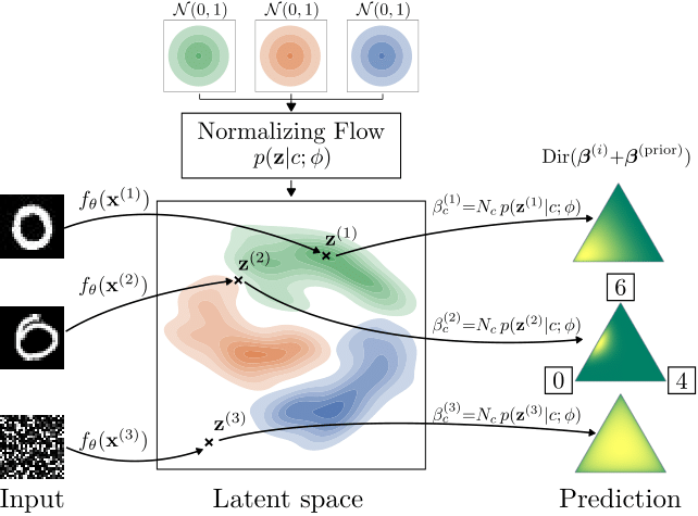
From (Charpentier et al., 2020):
Each input $\boldsymbol{x^{(i)}}$ is mapped to their to their latent vector $\boldsymbol{z^{(i)}}$. The normalizing flow component learns flexible density functions \(P(\boldsymbol{z} \vert y=c, \boldsymbol{\phi})\), for which we evaluate their densities at the positions of the latent vectors $\boldsymbol{z^{(i)}}$. These densities are used to parameterize a Dirichlet distribution for each data point, as seen on the right hand side. Higher densities correspond to higher confidence in the Dirichlet distributions.
We can observe that the out-of-distribution sample $\boldsymbol{x^{(3)}}$ is mapped to a point with (almost) no density, and hence its predicted Dirichlet distribution has very high epistemic uncertainty. On the other hand, $\boldsymbol{x^{(2)}}$ is an ambiguous example that could depict either the digit 0 or 6. This is reflected in its corresponding Dirichlet distribution, which has high aleatoric uncertainty (as the sample is ambiguous), but low epistemic uncertainty (since it is from the distribution of hand-drawn digits). The unambiguous sample $\boldsymbol{x^{(1)}}$ has low overall uncertainty.
Learning
Training loss is similar to the ELBO loss used in variational inference for Eq.(\ref{eq:variational_inference}) by optimizing jointly over the neural network parameters $\boldsymbol{\theta}$ and normalizing flow parameters $\boldsymbol{\phi}$:
\[\begin{equation} \mathcal{L}_{\textrm{PostNet}}(\boldsymbol{\theta}, \boldsymbol{\phi}) = \mathbb{E}_{p(\boldsymbol{x}, y)} \Big [ \mathbb{E}_{q_{\boldsymbol{\theta}, \boldsymbol{\phi}}(\boldsymbol{\pi} \vert \boldsymbol{x})} \big [ - \log p(y \vert \boldsymbol{\pi}, \boldsymbol{x}) \big ] + \mathrm{KL} \big (q_{\boldsymbol{\theta}, \boldsymbol{\phi}}(\boldsymbol{\pi} \vert \boldsymbol{x})~\vert \vert~p(\boldsymbol{\pi} \vert \boldsymbol{x}) \big ) \Big] \end{equation}\]Measuring uncertainty
(Charpentier et al., 2020) evaluate many uncertainty tasks such as misclassification detection, confidence calibration, OOD detection and robustness to dataset shift. In each task, they use 2 different measures: one for aleatoric uncertainty and one for epistemic uncertainty
- Misclassification detection: MCP as aleatoric measure; \(\max_c \alpha_c\) as epistemic measure, which corresponds to the logits of the predictive class,
- Confidence calibration: they simply use the Brier score with the output of the neural network,
- OOD detection: MCP as aleatoric measure; $\alpha_0$ as epistemic measure,
- Robustness to dataset shifts: obviously the accuracy on the shifted dataset.
Summary and Discussion
In light of this thorough analysis of each approach, we can see that most of them actually define similarly its loss.
| Method | Loss | \(\alpha\)-parametrization | OOD training data |
|---|---|---|---|
| Prior Networks | \(\mathcal{L}_{\textrm{RKL-PN}}(\boldsymbol{\theta}) = \mathbb{E}_{p(\boldsymbol{x} \vert i)} \Big [\sum_{c=1}^C p(y=c \vert \boldsymbol{x}) \cdot \textrm{KL} \big ( \textrm{Dir} ( \boldsymbol{\pi} \vert \boldsymbol{x}, \boldsymbol{\theta} ) ~\vert \vert~ \textrm{Dir} ( \boldsymbol{\pi} \vert \boldsymbol{\beta}^{(c)}_{\textrm{in}}) \big ) \Big ])\) \(~~~\quad\quad\quad\quad\quad + \gamma \cdot \mathbb{E}_{p(\boldsymbol{x} \vert o)} \Big [\sum_{c=1}^C p(y=c \vert \boldsymbol{x}) \cdot \textrm{KL} \big ( \textrm{Dir} ( \boldsymbol{\pi} \vert \boldsymbol{x}, \boldsymbol{\theta} ) ~\vert \vert~ \textrm{Dir} ( \boldsymbol{\pi} \vert \boldsymbol{\beta}^{(c)}_{\textrm{out}}) \big ) \Big ]\) |
\(\alpha_c = e^{f_c(\boldsymbol{x}, \boldsymbol{\theta})}\) | Yes |
| Max-Gap Prior Networks | \(\mathcal{L}_{\textrm{Max-PN}}(\boldsymbol{\theta}) = \mathbb{E}_{p(\boldsymbol{x}, y \vert i)} \Big [ - \log p(y \vert \boldsymbol{x}, \boldsymbol{\theta}) - \frac{\lambda_{\textrm{i}}}{C} \sum_{c=1}^C \sigma(\alpha_c) \Big ]\) \(\quad\quad\quad\quad\quad\quad\quad + \gamma \cdot \mathbb{E}_{p(\boldsymbol{x}, y \vert o)} \Big [ \mathcal{H} \big [p(y \vert \boldsymbol{x}, \boldsymbol{\theta}) \big ] - \frac{\lambda_{\textrm{o}}}{C} \sum_{c=1}^C \sigma(\alpha_c) \Big ]\) |
\(\alpha_c = e^{f_c(\boldsymbol{x}, \boldsymbol{\theta})}\) | Yes |
| Evidential Networks | \(\mathcal{L}_{\textrm{ENN}}(\boldsymbol{\theta}) = \mathbb{E}_{p(\boldsymbol{x}, y)} \Big [\int \vert \vert \boldsymbol{y} - \boldsymbol{\pi} \vert \vert^2 \cdot p(\boldsymbol{\pi} \vert \boldsymbol{x}, \boldsymbol{\theta}) d\boldsymbol{\pi} + \lambda_t \cdot \textrm{KL} \big ( \textrm{Dir} ( \boldsymbol{\pi} \vert \tilde{\boldsymbol{\alpha}} ) ~\vert \vert~ \textrm{Dir} (\boldsymbol{\pi} \vert \mathbf{u}) \big ) \Big ]\) | \(\alpha_c = \textrm{ReLU} \big ( f_c(\boldsymbol{x}, \boldsymbol{\theta}) \big ) + 1\) | No |
| Generative Evidential Networks | \(\mathcal{L}_{\textrm{GEN}}(\boldsymbol{\theta}) = - \sum_{c=1}^C \Big (\mathbb{E}_{p(\boldsymbol{x} \vert c, i)} \big [\log \sigma ( f_c(\boldsymbol{x}, \boldsymbol{\theta})) \big ] + \mathbb{E}_{p(\boldsymbol{x} \vert o)} \big [\log \big ( 1 - \sigma ( f_c(\boldsymbol{x}, \boldsymbol{\theta})) \big ) \big ] \Big )\) \(\quad\quad\quad\quad\quad\quad\quad\quad\quad\quad+ \lambda \cdot \mathbb{E}_{p(\boldsymbol{x},y \vert i)} \Big [ \textrm{KL} \big ( \textrm{Dir} (\boldsymbol{\pi}_{-y} \vert \boldsymbol{\alpha}_{-y} )~\vert \vert~ \textrm{Dir} (\boldsymbol{\pi}_{-y} \vert \mathbf{u}) \big ) \Big ]\) |
\(\boldsymbol{\alpha} = e^{f(\boldsymbol{x}, \boldsymbol{\theta})} + 1\) | No |
| Variational Inference | \(\mathcal{L}_{\textrm{VI}}(\boldsymbol{\theta}) = \mathbb{E}_{p(\boldsymbol{x}, y)} \Big [ \mathbb{E}_{q_{\boldsymbol{\theta}}(\boldsymbol{\pi} \vert \boldsymbol{x})} \big [ - \log p(y \vert \boldsymbol{\pi}, \boldsymbol{x}) \big ] + \mathrm{KL} \big (q_{\boldsymbol{\theta}}(\boldsymbol{\pi} \vert \boldsymbol{x})~\vert \vert~p(\boldsymbol{\pi} \vert \boldsymbol{x}) \big ) \Big]\) | \(\alpha_c = e^{f_c(\boldsymbol{x}, \boldsymbol{\theta})}\) | No |
| Posterior Networks | \(\mathcal{L}_{\textrm{PostNet}}(\boldsymbol{\theta}, \boldsymbol{\phi}) = \mathbb{E}_{p(\boldsymbol{x}, y)} \Big [ \mathbb{E}_{q_{\boldsymbol{\theta}, \boldsymbol{\phi}}(\boldsymbol{\pi} \vert \boldsymbol{x})} \big [ - \log p(y \vert \boldsymbol{\pi}, \boldsymbol{x}) \big ] + \mathrm{KL} \big (q_{\boldsymbol{\theta}, \boldsymbol{\phi}}(\boldsymbol{\pi} \vert \boldsymbol{x})~\vert \vert~p(\boldsymbol{\pi} \vert \boldsymbol{x}) \big ) \Big]\) | \(\alpha_c = \textrm{ReLU} \big ( f_c(\boldsymbol{x}, \boldsymbol{\theta}) \big ) + 1\) | No |
As already pointed out in Section 7, the ELBO loss \(\mathcal{L}_{\textrm{VI}}\) and the in-domain loss term in \(\mathcal{L}_{\textrm{RKL-PN}}\) are actually similar. Posterior networks also use a KL-divergence minimization loss \(\mathcal{L}_{\textrm{PostNet}}\) with the specifity of optimizing normalizing flow parameters as well.
\(\Rightarrow\) How to induce such desired behavior when training Dirichlet networks?
Going back to our first motivational question, we can distinguish 2 types of approach:
- force explicitely low concentration parameters for out-of-distribution samples, either by specifying a uniform target (Malinin & Gales, 2019) or by adding an explicit regularization on logits in the training loss (Nandy et al., 2020);
- incorporate a density modeling to account for out-of-distribution samples during training, either implicitely such as in noise contrastive estimation (Sensoy et al., 2020) or explicitely with a density estimator based on normalizing flows (Charpentier et al., 2020).
Neither (Sensoy et al., 2018),(Joo et al., 2020) or (Joo et al., 2020) account for the existence of out-domain samples in their framework. It is unlikely their method will accurately predict a high epistemic uncertainty for this kind of inputs.
\(\Rightarrow\) What measure should we use for each type of uncertainty?
Except the decomposition proposed by (Malinin & Gales, 2018) of uncertainty into total, aleatoric and epistemic obtainable via mutual information, there have not been many works on defining a proper uncertainty measure. Many approaches rely simply on MCP or the predictive entropy as their training loss often induce out-of-distribution inputs to have either small logits or high entropy.
However, in light of the previous decomposition, it theorically does not seems appropriate to use MCP/predictive entropy to measure OOD detection or misclassification detection. Indeed, these metrics corresponds to measuring the total uncertainty while evaluated tasks involve either aleatoric uncertainty or epistemic uncertainty.
Nevertheless, the correct results reported in papers may be explained as follow. We expect misclassifications to have high aleatoric uncertainty. As correct predictions and misclassifications are both in-domain samples, we may also expect them to have negligible epistemic uncertainty. That implies that a measure of total uncertainty will mostly be influenced by aleatoric uncertainty. Hence, as we do not include OOD samples when evaluating misclassification detection, a measure of total uncertainty will be able to perform correctly. Regarding OOD detection, the number of in-domain misclassifications is often very low due to high predicitive performances. Hence, confusing misclassifications with OOD samples will have a nearly negligible impact on average scores.
References
- K. P. Murphy. (2013). Machine learning : A Probabilistic Perspective. MIT Press.
- B. Lakshminarayanan, A. Pritzel, & C. Blundell. (2017). Simple and Scalable Predictive Uncertainty Estimation using Deep Ensembles. In Advances in Neural Information Processing Systems.
- Y. Gal, & Z. Ghahramani. (2016). Dropout as a Bayesian Approximation: Representing Model Uncertainty in Deep Learning. In Proceedings of the International Conference on Machine Learning.
- A. Malinin, & M. Gales. (2018). Predictive Uncertainty Estimation via Prior Networks. In Advances in Neural Information Processing Systems.
- M. Sensoy, L. Kaplan, & M. Kandemir. (2018). Evidential Deep Learning to Quantify Classification Uncertainty. In Advances in Neural Information Processing Systems.
- A. Malinin, & M. Gales. (2019). Reverse KL-Divergence Training of Prior Networks: Improved Uncertainty and Adversarial Robustness. In Advances in Neural Information Processing Systems.
- W. Chen, Y. Shen, W. Wang, & H. Jin. (2019). A Variational Dirichlet Framework for Out-of-Distribution Detection. ArXiv-Preprint.
- M. Sensoy, L. Kaplan, F. Cerutti, & M. Saleki. (2020). Uncertainty-Aware Deep Classifiers using Generative Models. In Proceedings of the AAAI Conference on Artificial Intelligence.
- T. Joo, U. Chung, & M.-G. Seo. (2020). Being Bayesian about Categorical Probability. In Proceedings of the International Conference on Machine Learning.
- J. Nandy, W. Hsu, & M.-L. Lee. (2020). Towards Maximizing the Representation Gap between In-Domain and Out-of-Distribution Examples. In Advances in Neural Information Processing Systems.
- B. Charpentier, D. Zügner, & S. Günnemann. (2020). Posterior Network: Uncertainty Estimation without OOD Samples via Density-Based Pseudo-Counts. In Advances in Neural Information Processing Systems.
- S. Depeweg, J. M. Hernández-Lobato, F. Doshi-Velez, & S. Udluft. (2018). Decomposition of Uncertainty in Bayesian Deep Learning for Efficient and Risk-sensitive Learning. In Proceedings of the International Conference on Machine Learning.
- D. Hendrycks, M. Mazeika, & T. Dietterich. (2019). Deep Anomaly Detection with Outlier Exposure. In Proceedings of the International Conference on Learning Representations.
- A. Josang. (2016). Subjective Logic: A Formalism for Reasoning Under Uncertainty. Springer.
- A. P. Dempster. (2008). A Generalization of Bayesian Inference. Springer.
- B. Lakshminarayanan, & S. Mohamed. (2017). Learning in Implicit Generative Models. ArXiv-Preprint.
- M. U. Gutmann, & A. Hyvärinen. (2012). Noise-contrastive estimation of unnormalized statistical models, with applications to natural image statistics. In Journal of Machine Learning Research.
- D. Rezende, & S. Mohamed. (2015). Variational Inference with Normalizing Flows. In Proceedings of the International Conference on Machine Learning.